Death of the sampling theorem?

tl;dr:

A team from Columbia University led by Ken Shepard and Rafa Yuste claims to beat the 100 year old Sampling Theorem [1,2]. Apparently anti-aliasing filters are superfluous now because one can reconstruct the aliased noise after sampling. Sounds crazy? Yes it is. I offer $1000 to the first person who proves otherwise. To collect your cool cash be sure to read to the end.

“Filter before sampling!”

This mantra has been drilled into generations of engineering students. “Sampling” here refers to the conversion of a continuous function of time into a series of discrete samples, a process that happens wherever a computer digitizes a measurement from the world. “Filter” means the removal of high-frequency components from the signal. That filtering process, because it happens in the analog world, requires real analog hardware: so-called “anti-aliasing” circuits made of resistors, capacitors, and amplifiers. That can be tedious, for example because there isn’t enough space on the electronic chips in question. This is the constraint considered by Shepard’s team, in the context of a device for recording signals from nerve cells [2].

Now these authors declare that they have invented an “acquisition paradigm that negates the requirement for per-channel anti-aliasing filters, thereby overcoming scaling limitations faced by existing systems” [2]. Effectively they can replace the anti-aliasing hardware with software that operates on the digital side after the sampling step. “Another advantage of this data acquisition approach is that the signal processing steps (channel separation and aliased noise removal) are all implemented in the digital domain” [2].

This would be a momentous development. Not only does it overturn almost a century of conventional wisdom. It also makes obsolete a mountain of electronic hardware. Anti-alias filters are ubiquitous in electronics. Your cell phone contains multiple digital radios and an audio digitizer, which between them may account for half a dozen anti-alias circuits. If given a chance today to replace all those electronic components with a few lines of code, manufacturers would jump on it. So this is potentially a billion dollar idea.

Unfortunately it is also a big mistake. I will show that these papers do nothing to rattle the sampling theorem. They do not undo aliasing via post-hoc processing. They do not obviate analog filters prior to digitizing. And they do not even come close to the state of the art for extracting neural signals from noise.

Why aliasing is bad for you

[skip if you know the answer]

Sampling is that critical step in data acquisition when a continuous signal gets turned into a discrete series of numbers. Most commonly the continuous signal is a voltage trace, and it gets sampled and digitized at regular time intervals by an electronic circuit called “analog-to-digital converter” (Fig 1). Naively one would think that sampling incurs a loss of information. After all, the continuous voltage curve has “infinitely many” points on it, but after sampling we are left with observing only a finite number of those. The infinite number of points between the samples must therefore be lost. Here is where the Sampling Theorem [3,4] makes a remarkable statement: Under suitable conditions the discrete samples contain all the information needed to perfectly reconstruct the continuous voltage function that produced them. In that case there is no information loss from sampling.

Those suitable conditions are simple: The input signal should vary sufficiently slowly so the sequence of samples captures it well. Specifically the signal should have no sinusoidal components at frequencies above the so-called Nyquist frequency, which is equal to half the sampling rate:

                                  (1)

For example, if the digitizer takes samples at a rate of 10,000 Samples/s, the input signal should have no components above 5,000 Hz. What happens if the input signal varies faster than that? Those frequency components cannot be reconstructed from the samples, because their origin is perfectly ambiguous (Fig 1).

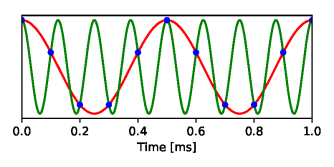
Fig 1: Aliasing. A sine wave with a frequency of 2 kHz (red) gets sampled at a rate of 10 kS/s (blue dots). Another sine wave with frequency 8 kHz produces the exact same sequence of samples. So after sampling one cannot reconstruct whether the original signal was at 2 kHz or at 8 kHz.

The same set of samples may have resulted from a signal below the Nyquist frequency or from any number of possible signals above the Nyquist frequency. This phenomenon is called “aliasing”, because a high-frequency signal can masquerade in the sampled waveform as a low-frequency signal [5]. If no other constraints are known about the input signal, then aliasing leads to information loss, because the input can no longer be reconstructed from the samples.

How to avoid aliasing? Simply make sure to eliminate frequency components above the Nyquist rate from the analog signal before the sampling step. Most commonly this is done with an electronic “low pass” filter that allows low frequencies through but cuts out high frequencies. A great deal of engineering expertise has gone into designing these filters because of their ubiquitous applications. So the usual design process for an acquisition system is this (Fig 2):

1. Determine the bandwidth of the signal you want to observe, namely the highest frequency component you will want to reconstruct for your purpose. This is the Nyquist frequency of your system.
2. Send the signal through a low-pass filter that removes all frequencies above .
3. Sample the output of the filter at a rate .

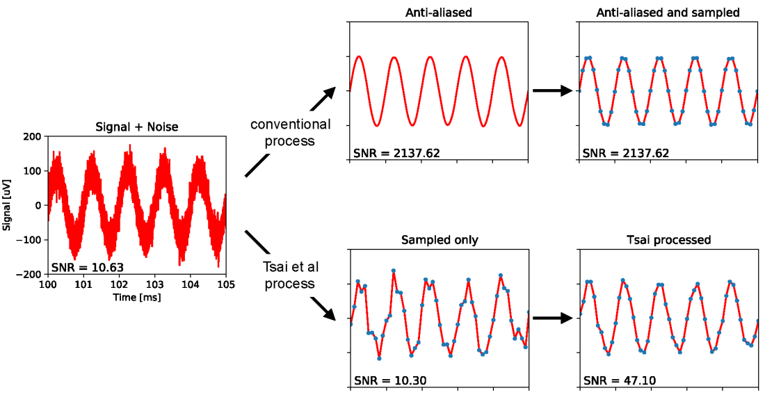
Fig 2: Comparison of conventional data acquisition with the process followed by Tsai et al. Left: A sine wave at 1 kHz with 200 µV peak-to-peak amplitude, like in the Tsai et al test recordings. Added is Gaussian white noise with a bandwidth of 1 MHz and 21.7 µV rms amplitude. Top: The standard approach is to apply an anti-alias filter with 5 kHz cutoff frequency, which eliminates most of the noise and thus improves the signal-to-noise power ratio (SNR) by a factor of 200. This signal is then sampled at 10 kS/s. Bottom: In the approach followed by Tsai et al the signal is sampled directly, thus leaving the same poor SNR. This is followed by a digital processing step that provides a modest increase in SNR. All data and processing are simulated with code found in [6].

What Tsai et al claim

Let us consider now the specific situation in Tsai et al’s reports. They want to record electric signals from neurons, which requires a bandwidth of . So they choose to sample the signal at a rate of = 10 kS/s (kilosamples per second). Unfortunately the desired neural signal is corrupted by broadband thermal noise, an unavoidable byproduct of the recording technology. The noise has a spectrum that reaches up to 1 MHz with a typical root-mean-square (rms) amplitude of 21.7 µV. The authors approximate it as Gaussian white noise, which means the noise has constant power density up to the 1 MHz cutoff. (References for these numbers: p.5 and Fig 11 of [1]; p.2, 5, 9 and Suppl Fig 2e of [2]).

The conventional procedure would be to pass signal + noise through an analog anti-alias filter with 5 kHz cutoff (Fig 2). That would leave the neural signal unaffected, while reducing the amount of noise power by a factor of 200, because the spectrum is cut from 1 MHz bandwidth to just 5 kHz. The remaining noise below the Nyquist frequency would thus have a rms amplitude of only 21.7 µV/ = 1.53 µV rms. This amount of thermal noise is perfectly innocuous, smaller than other noise sources in the experiment. Then the signal can get sampled at a sampling rate of 10 kS/s.

Instead of following this path, the authors leave out the anti-alias filter entirely and sample the broadband signal + noise directly. There are technical reasons for omitting the filter circuits, having to do with the tight space constraints on silicon devices in this recording method, and they are well explained in the article [1]. But as a consequence all the noise power up to the 1 MHz cutoff now appears in the sampled signal via aliasing. Effectively every sample is contaminated by Gaussian noise of 21.7 µV rms. That noise level is unacceptable, because one would like to resolve neural signals of that same amplitude or less. For reference, some systems in popular use for multi-neuron recording have noise levels below 4 µV [7,8].

Here comes the startling “innovation” from Tsai et al: They say that one can apply a clever data processing algorithm after sampling to reconstruct the original broadband noise, subtract the noise from the sampled data, and thus remove it, leaving pure signal behind. Here are some relevant quotes, in addition to those already cited above: “we can digitally reconstruct the spectral contributions originating from the under-sampled thermal noise, then remove them from the sparsely-sampled channel data, thereby minimizing the effects of aliasing, without using per-channel anti-aliasing filters” [2]. And “We present a multiplexing architecture without per-channel antialiasing filters. The sparsely sampled data are recovered through a compressed sensing strategy, involving statistical reconstruction and removal of the undersampled thermal noise” [1].

What evidence do they offer for this claim? There is only one experiment that actually measures the noise reduction using ground truth data. The authors record a sine wave test signal at 1 kHz frequency and 200 µV peak-to-peak amplitude. Then they apply their data processing scheme to “remove thermal noise”. The output signal does look cleaner than the input (Fig 2e of [2]; see also simulation in Fig 2). Quantitatively, the noise was reduced from 21.7 μV rms to 10.02 μV. This is a rather modest improvement of the signal-to-noise power ratio (SNR) by a factor of 4.7 (more on that below). A proper anti-alias filter before sampling, or the advertised removal of aliased noise after sampling, should have increased the SNR by a factor of 200. (References for results quoted here: Fig 2e-f of [2] and Fig 7 of [1].)

Why the scheme of Tsai et al cannot work in principle

Before getting into the nitty gritty of the data processing scheme proposed in these papers, it is worth contemplating why the scheme cannot work in principle. Most prominently: If true, this claim would overturn the Sampling Theorem that generations of engineering students learned in college. The white-noise signal in these experiments is sampled at a rate 200 times lower than what the Sampling Theorem requires to allow reconstruction. So why do Tsai et al think the scheme could work anyway?

The authors claim that the aliased high-frequency noise somehow retains a fingerprint of having been aliased, which allows you to remove it after the fact: “Taking advantage of the foregoing characteristics, we can digitally reconstruct the spectral contributions originating from the under-sampled thermal noise, then remove them from the sparsely-sampled channel data, thereby minimizing the effects of aliasing” [2]. It is hard to see what characteristics those might be. This can be appreciated most easily in the time domain. Gaussian white noise with a 1 MHz bandwidth can be instantiated by a time series of samples drawn independently from an identical Gaussian distribution at 2 MS/s. Now take this time series and subsample it at 10 kS/s, i.e. pick only every 200^th of the original samples. You will again get independently and identically distributed samples, i.e. Gaussian white noise at 10 kS/s. Nothing about this series of samples reveals that it started out from a high frequency source. It remains perfectly aliased.

Fig 3: Sampling Gaussian white noise. Left: Gaussian white noise (red line) with an rms amplitude 21.7 µV and a bandwidth of 1 MHz gets sampled at a rate of 10 kS/s (blue dots). Right: The sampled signal on a 200x wider time scale. This signal is again Gaussian white noise, with the same amplitude distribution (margin plots), but a bandwidth of 5 kHz.

The authors also claim that their algorithm “avoids aliasing using concepts from compressed sensing” [2] to reconstruct the Gaussian white noise. The principle of compressed sensing is that one can sample a signal without loss at less than the Nyquist rate as long as it exhibits known regularities. In particular the signal should have a sparse distribution along certain directions in data space, which offers opportunities for compression [9]. This is the case for many natural signal sources, like photographic images. Unfortunately Gaussian white noise is the ultimate pattern-free non-compressible signal. The probability distribution for this signal is a round and squishy Gaussian sphere that looks the same from all directions in data space, and simply offers no purchase for any compression strategies. Of course the neural signals riding on top of the noise do contain some statistical regularities (more on that below). But those don’t help in reconstructing the noise.

How the scheme of Tsai et al fails in practice

I coded the algorithm that Tsai et al describe [6]. When presented with a simulation of the authors’ test (200 µV sine wave in 21.7 µV noise) it returns the cleaned-up sine wave with only 10.2 µV noise (Fig 2), awfully close to the Tsai et al report of 10.02 µV. This suggests that I emulated the scheme correctly.

Along the way I encountered what looks like the key mathematical mistake. It relates to the authors’ belief that the undersampled noise retains some signature that results from aliasing. Referring to the Fourier representation of Gaussian white noise they write (section III.G of [2]) “the Fourier space vector angles for thermal noise (of infinite length) has a uniform distribution with zero mean. Again, any departure from this ideal in finite-length signals is averaged out by aliasing, when the contents are folded down into the first Nyquist zone (Fig. 6(a)), causing the angles to converge to zero.” And similarly “the spectral angles converge to zero in the aliased version of the thermal noise” (p.9 bottom left of [1]). This is wrong. The phase angles of the Fourier vectors in question here have a uniform circular distribution; that distribution has no mean angle. After averaging some of these vectors via aliasing, the phase of the average vector again has a uniform circular distribution. This proves in Fourier space what is more easily appreciated in direct space: subsampling Gaussian white noise leaves you again with Gaussian white noise (Fig 3). The rationale for the Tsai algorithm is based on this erroneous conception that phase angles somehow average to zero.

So how does the Tsai algorithm clean up a sinusoid test signal? That’s not really hard to do. If you know the signal is a pure sinusoid there are only 3 unknowns: amplitude, phase, and frequency. Obviously you can extract those 3 unknowns from the 10,000 noisy samples you get every second. It can be done much more efficiently: find the largest Fourier component in the sampled recording, and set all the others to zero. This removes noise almost completely (for more on this see [6]). The Tsai algorithm does a little bit of that, suppressing the off-peak frequencies in the Fourier transform more than on-peak, and so it gets some amount of noise suppression for sine waves (see also Fig 9 of [1]). As we will see, that performance does not extend to realistic signals.

What would be a reasonable processing scheme?

The sine-wave example introduces how one should really think about post-hoc data processing: Trying to reconstruct the aliased noise is hopeless for all the reasons explained above. One simply has to accept the level of noise that results from all the aliasing. Instead one should focus on properties of the signal that we want to separate from the noise. If the signal has statistical regularities then we can use those in our favor. The sine wave of course is extremely regular, and thus we can extract it from the noise to almost infinite precision. More generally we may have some partial knowledge of the signal statistics, for example the shape of the power spectrum. Neural action potentials have frequency components up to ~5 kHz, but their spectrum is not flat over that whole range (Fig 4).

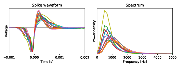
Fig 4. Left: Average waveform of the action potential for 15 retinal ganglion cells of the mouse [10]. Right: Power spectra derived from these spike shapes.

Suppose we know the power spectrum of the signal and it differs from the spectrum of the noise, how should we process the sampled data to optimally reconstruct the signal? This is a classic problem taught in signal processing courses. The optimal linear filter for a least-squared-error reconstruction is called the “Wiener filter” [11], which essentially suppresses frequency components where the noise is relatively larger. Now the Tsai algorithm is a non-linear operation (see details in [6]), so in principle it might outperform the Wiener filter. Also, because of the nonlinearity one cannot use the algorithm’s performance with sinusoid signals (see above) to predict what it might do with more general signals. So I compared the Tsai algorithm to the classic Wiener filter, using various assumptions for the signal spectrum. In particular the signal was restricted below a cutoff frequency ranging from 100 Hz to 5000 Hz, whereas the noise had a uniform spectrum across the 5 kHz band:

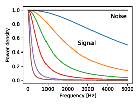
Fig 5. Power spectra of Signal (colored lines) and Noise (black) used in the simulations of Fig 6. Noise is Gaussian and white across the 5 kHz band. Signal is derived from a Gaussian white process passed through a single-pole low-pass filter with cutoff frequencies at 5000, 2000, 1000, 500, 200, 100 Hz.

For each of these combinations of signal and noise, I applied either the Wiener filter or the Tsai algorithm, and measured the signal-to-noise ratio (SNR) in the resulting output (Fig 6).

Fig 6. Comparing how the Tsai algorithm and the Wiener filter affect the signal-to-noise ratio. Each panel corresponds to a different power spectrum for the signal (see Fig 5). Signal and noise were mixed at different SNRs, plotted on the horizontal axis. The result was passed through either a Wiener filter or the Tsai algorithm, and the SNR of the output signal is plotted on the vertical axis. Red: Wiener filter; green: Tsai algorithm; dotted: identity.

As expected, the Wiener filter always improves the SNR (compare red curve with the dotted identity), and more so the more the spectra of signal and noise are different (panels top left to bottom right). Under all the conditions I tested, the Wiener filter outperforms the Tsai algorithm in improving the SNR (compare red and green curves). Moreover, under many conditions the Tsai algorithm actually degrades the SNR, meaning it is worse than doing nothing (compare green and dotted curves). Given that the algorithm is based on mathematical errors, this is not surprising.

There are more sophisticated schemes for noise suppression than the Wiener filter. For example we know that the neural recordings of interest are a superposition of pulse-like events – the action potentials – whose pulse shapes are described by just a few parameters. Under that statistical model for the signal one can develop algorithms that optimally estimate the spike times from noisy samples. This is a lively area of investigation [12–15].

Why this matters for neuroscience

There is great push from the neuroscience community for increasing the number of neurons we can monitor simultaneously. Progress in this area has been exponential but rather slow, with a doubling time of 7 years [16]. Several projects are afoot to accelerate this by building large-scale CMOS devices with thousands of densely spaced electrodes and multiplexing switches [2,7,17–19]. Taking the manufacture of such devices to the stage where real functioning electrode arrays are distributed to researchers is an expensive undertaking, on the scale of millions of dollars. If the success of such a device is predicated on erroneous beliefs about aliasing and undue expectations from software, this could lead to expensive failures and waste of precious resources.

A painful experience of this type was the Fromherz array [20]. Designed in a collaboration with Siemens, at a cost in the millions of DM, this was the largest electrode array of its time, with 16384 sensors on a 7.8 µm pitch. For all the usual reasons the designers omitted the anti-alias filters. Aliasing and other imperfections ended up producing a noise level of 250 µV [21], unsuitable for any interesting experiments, and the device has never been used productively. This outcome could have been predicted by simple calculations.

If one treats the consequences of aliasing rationally ahead of time, then useful compromises are possible. For example, a recent silicon prong device also uses multiplexing switches without anti-alias filters [18]. But the undersampling ratio is only 8:1, which leads to a tolerable level of excess noise [22]. When combined with proper signal reconstruction such a scheme can work productively.

Who reviewed this work?

As so often, one does have to ask: How did these dramatic claims get through peer review? Given the obvious conflict with the Sampling Theorem, weren’t some eyebrows raised in the process? Who reviewed these submissions anyway? Well, I did. For a different journal, where the manuscript ultimately got rejected. Before that happened there was a lengthy exchange with the authors, including my challenge to remove aliased noise from a simulated recording (see below, minus the cash prize). The authors accepted the challenge as a reasonable test of the algorithm, but their signal estimation thoroughly failed the test. Somehow that did not shake their confidence, and they presented the exact same claims to two other journals. Those journals, presumably after so-called peer review, were happy to comply.

How to win $1000

Of course it is possible that I misunderstood the Tsai algorithm, or that against all odds there exists a different scheme to reconstruct aliased white noise after sampling. To stimulate creative work in this area I offer this challenge: If you can do what Tsai et al claim is possible, I will give you $1000. Here is how it works:

You start by sending me $10 for “shipping and handling” (Paypal meister4@mac.com, thank you). In return I send you a data file containing the result of sampling Signal + Noise at 10 kS/s, where Signal is band-limited below the Nyquist frequency of 5 kHz, and Noise is Gaussian white noise with a bandwidth of 1 MHz. You will use the Tsai algorithm or any scheme of your choosing to remove the aliased Noise as much as possible, and send me back a data file containing your best estimate of the Signal. If you can improve the signal-to-noise power ratio (SNR) in this estimate by a factor of 2 or more, I will pay you $1000. Note that a proper anti-alias filter can increase the SNR by a factor of 200 (Fig 2), and Tsai et al claim to increase it by a factor >4, so I am just asking for a tiny bit of noise removal here. For more technical details see code and comments in my Jupyter Notebook [6].

A few more rules: The offer is open for 30 days from the date of this post. Only the first qualifying entry wins. You must reveal the algorithm used so I may reproduce its performance. After beating your head against the Sampling Theorem you may decide to try something different, like a cryptographic attack on the random seed I used to produce the data file. While I would be curious about such alternate solutions, I won’t pay $1000 for that but only refund your $10.

Finally, I don’t want to take money from beginners. Before you send me $10, be sure to test your algorithm extensively using the code in my Jupyter Notebook [6]: That’s what I will use to evaluate it.

Bottom line

Until someone cashes my $1000 check, the conclusions are:

• Tsai et al built a digitizer that lacks anti-alias filters, and as a result accepts ~200 times more noise power from thermal fluctuations than would be necessary.
• Their post-sampling algorithm does nothing to reverse the effects of aliasing. At best it is an attempt to separate the desired signal from the corrupting aliased noise. Unfortunately the algorithm is based on mathematical errors.
• Better algorithms for separating signal from white noise are well known. For sinusoid signals (the case documented by the authors) that separation is trivial. For band-limited signals whose power spectrum differs from that of the noise, the Wiener filter is a classic solution. Under all conditions tested, the Wiener filter does better than the Tsai algorithm. Under many conditions the Tsai algorithm is worse than doing nothing.
• For the time being I suggest that hardware designers should stick to the ancient wisdom of “filter before sampling!”

Bibliography

1. Tsai D, Yuste R, Shepard KL. Statistically Reconstructed Multiplexing for Very Dense, High-Channel-Count Acquisition Systems. IEEE Trans Biomed Circuits Syst. 2017; 1–11. doi:10.1109/TBCAS.2017.2750484
2. Tsai D, Sawyer D, Bradd A, Yuste R, Shepard KL. A very large-scale microelectrode array for cellular-resolution electrophysiology. Nat Commun. 2017;8: 1802. doi:10.1038/s41467-017-02009-x
3. Shannon CE. Communication in the Presence of Noise. Proc IRE. 1949;37: 10–21. doi:10.1109/JRPROC.1949.232969
4. Nyquist–Shannon sampling theorem. In: Wikipedia [Internet]. [cited 6 Mar 2018]. Available: https://en.wikipedia.org/wiki/Nyquist–Shannon_sampling_theorem
5. Aliasing. In: Wikipedia [Internet]. Available: https://en.wikipedia.org/wiki/Aliasing
6. Jupyter Notebook for Tsai et al Critique [Internet]. Available: https://github.com/markusmeister/Aliasing
7. Muller J, Ballini M, Livi P, Chen Y, Radivojevic M, Shadmani A, et al. High-resolution CMOS MEA platform to study neurons at subcellular, cellular, and network levels. Lab Chip. 2015;15: 2767–80. doi:10.1039/c5lc00133a
8. Du J, Blanche TJ, Harrison RR, Lester HA, Masmanidis SC. Multiplexed, high density electrophysiology with nanofabricated neural probes. PLoS One. 2011;6: e26204. doi:10.1371/journal.pone.0026204
9. Ganguli S, Sompolinsky H. Compressed Sensing, Sparsity, and Dimensionality in Neuronal Information Processing and Data Analysis. Annu Rev Neurosci. 2012; doi:10.1146/annurev-neuro-062111-150410
10. Krieger B, Qiao M, Rousso DL, Sanes JR, Meister M. Four alpha ganglion cell types in mouse retina: Function, structure, and molecular signatures. PLoS One. 2017;12: e0180091. doi:10.1371/journal.pone.0180091
11. Generalized Wiener filter. In: Wikipedia [Internet]. Available: https://en.wikipedia.org/wiki/Generalized_Wiener_filter
12. Ekanadham C, Tranchina D, Simoncelli EP. A unified framework and method for automatic neural spike identification. J Neurosci Methods. 2014;222: 47–55. doi:10.1016/j.jneumeth.2013.10.001
13. Pachitariu M, Steinmetz NA, Kadir SN, Carandini M, Harris KD. Fast and accurate spike sorting of high-channel count probes with KiloSort. In: Lee DD, Sugiyama M, Luxburg UV, Guyon I, Garnett R, editors. Advances in Neural Information Processing Systems 29. Curran Associates, Inc.; 2016. pp. 4448–4456. Available: http://papers.nips.cc/paper/6326-fast-and-accurate-spike-sorting-of-high-channel-count-probes-with-kilosort.pdf
14. Pillow JW, Shlens J, Chichilnisky EJ, Simoncelli EP. A model-based spike sorting algorithm for removing correlation artifacts in multi-neuron recordings. PLoS One. 2013;8: e62123. doi:10.1371/journal.pone.0062123
15. Chung JE, Magland JF, Barnett AH, Tolosa VM, Tooker AC, Lee KY, et al. A Fully Automated Approach to Spike Sorting. Neuron. 2017;95: 1381–1394.e6. doi:10.1016/j.neuron.2017.08.030
16. Stevenson IH, Körding KP. How advances in neural recording affect data analysis. Nat Neurosci. 2011;14: 139–42. doi:10.1038/nn.2731
17. Jun JJ, Steinmetz NA, Siegle JH, Denman DJ, Bauza M, Barbarits B, et al. Fully integrated silicon probes for high-density recording of neural activity. Nature. 2017;551: 232–236. doi:10.1038/nature24636
18. Raducanu BC, Yazicioglu RF, Lopez CM, Ballini M, Putzeys J, Wang S, et al. Time Multiplexed Active Neural Probe with 1356 Parallel Recording Sites. Sensors. 2017;17: 2388. doi:10.3390/s17102388
19. Researchers Revolutionize Brain-Computer Interfaces Using Silicon Electronics. In: Columbia Engineering [Internet]. [cited 8 Mar 2018]. Available: http://engineering.columbia.edu/news/ken-shepard-brain-computer-interface
20. Eversmann B, Jenkner M, Hofmann F, Paulus C, Brederlow R, Holzapfl B, et al. A 128×128 CMOS biosensor array for extracellular recording of neural activity. Ieee J Solid-State Circuits. 2003;38: 2306–2317. doi:10.1109/JSSC.2003.819174
21. Hutzler M, Lambacher A, Eversmann B, Jenkner M, Thewes R, Fromherz P. High-resolution multitransistor array recording of electrical field potentials in cultured brain slices. J Neurophysiol. 2006;96: 1638–45. doi:10.1152/jn.00347.2006
22. Dimitriadis G, Neto JP, Aarts A, Alexandru A, Ballini M, Battaglia F, et al. Why not record from every channel with a CMOS scanning probe? bioRxiv. 2018; 275818. doi:10.1101/275818